Contents:
Initial data-munging was done using a series of SQL queries. For direct further education entrants we took those who indicated that they had finished year 12 the year before and indicated that they were currently undertaking some form of teriary study. Gap-year students were derived by taking those who had completed year 12 the year before and indicated that they had defered further education and/or confirmed the following year that they had defered further education in the year previous.
Further education dropouts were taking by exploring if in any of the years under investigation they indicated they had withdrawn from their teriary education course. Gap-year returners composed those who had, at any time during the period of investigation indicated that they currently undertaking teriary education. SQL queries underlying theis subsetting are in .Rmd file associated with this file.
## Loading required package: DBI
## [1] "META1995"    "META1998"    "META2003"    "Student1995" "Student1998"
## [6] "Student2003"
The number of adolescence who directly entered university after high-school was 1723. The number of adolescents that took a gap-year (offered further education but defered) was 505.
The PISA database consistst on individuals who are the same age but may be in a veriety of year in school grades. In the current research we wanted to compare individuals in terms of years since high-school graduation rather than age in years. As such, we needed to rearrange the data.
The Satisfaction Items are (How satisfied are you with):
Items in bold are the ones used in the analysis.
## [1] "matching Features"
##      Variable                                             Label
## 2     stateid                                   State/Territory
## 4    schoolid                                         School ID
## 7         loc                                 MCEETYA Loc Class
## 8         sex                                 Sex of respondent
## 9       indig                                Final Indig Status
## 385    sisced     Expected educational level of student (ISCED)
## 395      escs                   Economic social cultural status
## 398    belong                Sense of belonging to school (WLE)
## 399    intmat                     Interest in mathematics (WLE)
## 400   instmot      Instrumental motivation in mathematics (WLE)
## 401   matheff                   Mathematics self-efficacy (WLE)
## 402    anxmat                         Mathematics anxiety (WLE)
## 403     scmat                    Mathematics self-concept (WLE)
## 407   complrn                        Competitive learning (WLE)
## 408   cooplrn                       Co-operative learning (WLE)
## 409  teachsup            Teacher support in maths lessons (WLE)
## 410   disclim       Disciplinary climate in maths lessons (WLE)
## 432    laa005                   A5 Respondent post-school plans
## 433    laa006                 A6 Parent post-school aspirations
## 434    laa007                  A7 Peer post-school expectations
## 670    laa025         A25 Self-assessment of literacy (English)
## 671    laa026     A26 Self-assessment of numeracy (Mathematics)
## 672    laa027                       A27 Overall self-assessment
## 729    lad001                              D1 Currently working
## 5196 xcsl2003            Derived: XCSL2003 Current school level
## 5364 xath2003           Derived: XATH2003 Living with parent(s)
## 10    pv1math                           Plausible value in math
## 15   pv1math1         Plausible value in math - Space and Shape
## 20   pv1math2 Plausible value in math- Change and Relationships
## 25   pv1math3             Plausible value in math - Uncertainty
## 30   pv1math4                Plausible value in math - Quantity
## 35    pv1read                        Plausible value in reading
## 40    pv1scie                        Plausible value in science
## 45    pv1prob                Plausible value in problem solving
## 238   st30q01                       Attitude enjoy reading Q30a
## 239   st30q02                              Attitude effort Q30b
## 240   st30q03                        Attitude look forward Q30c
## 241   st30q04                        Attitude enjoy Maths  Q30d
## 242   st30q05                             Attitude career  Q30e
## 243   st30q06                          Attitude interested Q30f
## 244   st30q07                       Attitude further study Q30g
## 245   st30q08                                Attitude job  Q30h
Percentage of missing data:
##             id         W1WORK      W1LEISURE    W1GET.ALONG         W1WAGE
##          0.000          0.008          0.007          0.007          0.012
##       W1SOCIAL W1INDEPENDENCE  W1CAREER.PROS  W1FUTURE.PROS    W1HOME.LIFE
##          0.006          0.007          0.018          0.018          0.007
##   W1LIVE.STAND        lbj003k        lbj003l    W1RESIDENCE     W1LIFE.SAT
##          0.007          0.039          0.104          0.007          0.008
##         W2WORK      W2LEISURE    W2GET.ALONG         W2WAGE       W2SOCIAL
##          0.004          0.001          0.000          0.008          0.000
## W2INDEPENDENCE  W2CAREER.PROS  W2FUTURE.PROS    W2HOME.LIFE   W2LIVE.STAND
##          0.001          0.007          0.012          0.001          0.000
##    W2RESIDENCE     W2LIFE.SAT         W3WORK      W3LEISURE    W3GET.ALONG
##          0.000          0.001          0.004          0.001          0.002
##         W3WAGE       W3SOCIAL W3INDEPENDENCE  W3CAREER.PROS  W3FUTURE.PROS
##          0.002          0.002          0.001          0.012          0.010
##    W3HOME.LIFE   W3LIVE.STAND    W3RESIDENCE     W3LIFE.SAT         W4WORK
##          0.002          0.001          0.000          0.002          0.092
##      W4LEISURE    W4GET.ALONG         W4WAGE       W4SOCIAL W4INDEPENDENCE
##          0.088          0.087          0.090          0.088          0.087
##  W4CAREER.PROS  W4FUTURE.PROS    W4HOME.LIFE   W4LIVE.STAND        lej005k
##          0.094          0.092          0.088          0.087          0.119
##        lej005l    W4RESIDENCE     W4LIFE.SAT         W5WORK      W5LEISURE
##          0.149          0.088          0.088          0.131          0.130
##    W5GET.ALONG         W5WAGE       W5SOCIAL W5INDEPENDENCE  W5CAREER.PROS
##          0.129          0.132          0.130          0.131          0.140
##  W5FUTURE.PROS    W5HOME.LIFE   W5LIVE.STAND        lfj003k        lfj003l
##          0.139          0.132          0.129          0.167          0.197
##    W5RESIDENCE     W5LIFE.SAT         W6WORK      W6LEISURE    W6GET.ALONG
##          0.130          0.130          0.198          0.196          0.194
##         W6WAGE       W6SOCIAL W6INDEPENDENCE  W6CAREER.PROS  W6FUTURE.PROS
##          0.194          0.194          0.194          0.199          0.199
##    W6HOME.LIFE   W6LIVE.STAND        lgj010k        lgj010l    W6RESIDENCE
##          0.194          0.194          0.211          0.232          0.196
##     W6LIFE.SAT         W7WORK      W7LEISURE    W7GET.ALONG         W7WAGE
##          0.196          0.263          0.261          0.261          0.264
##       W7SOCIAL W7INDEPENDENCE  W7CAREER.PROS  W7FUTURE.PROS    W7HOME.LIFE
##          0.261          0.260          0.265          0.265          0.260
##   W7LIVE.STAND        lhj001k        lhj001l    W7RESIDENCE     W7LIFE.SAT
##          0.260          0.283          0.294          0.261          0.261
##       W1STATUS       W2STATUS       W3STATUS       W4STATUS       W5STATUS
##          0.005          0.000          0.021          0.102          0.140
##       W6STATUS          group        stateid       schoolid            loc
##          0.206          0.000          0.000          0.000          0.000
##            sex         sisced          indig         laa005         laa006
##          0.000          0.000          0.000          0.000          0.000
##           escs         laa007         laa025         laa026         laa027
##          0.004          0.000          0.000          0.000          0.000
##       xcsl2003         lad001       xath2003         belong         intmat
##          0.000          0.000          0.000          0.001          0.001
##        instmot        matheff         anxmat          scmat        complrn
##          0.001          0.000          0.001          0.001          0.000
##        cooplrn       teachsup        disclim        pv1math       pv1math1
##          0.001          0.000          0.001          0.000          0.000
##       pv1math2       pv1math3       pv1math4        pv1read        pv1scie
##          0.000          0.000          0.000          0.000          0.000
##        pv1prob        st30q01        st30q02        st30q03        st30q04
##          0.000          0.002          0.003          0.008          0.006
##        st30q05        st30q06        st30q07        st30q08
##          0.002          0.005          0.002          0.004
## Pre-existing differences on matching variables:
##                Group Diff (SD Units)  t_value Significance
## W1WORK                     0.0423292  0.80173
## W1LEISURE                 -0.0597375 -1.15799
## W1GET.ALONG               -0.0154605 -0.30484
## W1WAGE                    -0.0172959 -0.33611
## W1SOCIAL                  -0.0786574 -1.52074
## W1INDEPENDENCE            -0.1083763 -2.11928            *
## W1CAREER.PROS              0.0633206  1.21527
## W1FUTURE.PROS             -0.0096553 -0.18671
## W1HOME.LIFE               -0.0572795 -1.13518
## W1LIVE.STAND              -0.0773963 -1.52578
## lbj003k                    0.0448033  0.82041
## lbj003l                    0.0079558  0.15081
## W1RESIDENCE               -0.0195720 -0.37747
## W1LIFE.SAT                -0.0965960 -1.92468
## W2WORK                     0.0802062  1.51447
## W2LEISURE                 -0.0585724 -1.15188
## W2GET.ALONG               -0.1321507 -2.68731            *
## W2WAGE                     0.0936169  1.82999
## W2SOCIAL                  -0.1246597 -2.50461            *
## W2INDEPENDENCE             0.0055059  0.10823
## W2CAREER.PROS              0.1244445  2.47189            *
## W2FUTURE.PROS              0.0009047  0.01782
## W2HOME.LIFE                0.0161713  0.31818
## W2LIVE.STAND               0.0005895  0.01151
## W2RESIDENCE                0.0094328  0.18419
## W2LIFE.SAT                 0.0160191  0.31888
## W3WORK                     0.0341866  0.61110
## W3LEISURE                 -0.1282585 -2.58317            *
## W3GET.ALONG               -0.1887982 -3.81479            *
## W3WAGE                    -0.0713672 -1.41442
## W3SOCIAL                  -0.0603746 -1.19190
## W3INDEPENDENCE            -0.1809012 -3.58326            *
## W3CAREER.PROS              0.0272382  0.53730
## W3FUTURE.PROS             -0.0633346 -1.21218
## W3HOME.LIFE               -0.1177495 -2.33902            *
## W3LIVE.STAND              -0.0768407 -1.51365
## W3RESIDENCE               -0.0322919 -0.64524
## W3LIFE.SAT                -0.1542453 -3.11274            *
## escs                      -0.1404837 -2.93409            *
## laa007                    -0.1382104 -2.59364            *
## laa025                    -0.0865514 -1.73553
## laa026                    -0.1690189 -3.22302            *
## laa027                    -0.0992775 -1.89248
## lad001                    -0.2100516 -4.14030            *
## belong                    -0.0216606 -0.42639
## intmat                     0.2027070  4.15895            *
## instmot                    0.1871466  3.71959            *
## matheff                    0.0960648  1.90415
## anxmat                    -0.0631447 -1.32567
## scmat                      0.2013838  3.96249            *
## complrn                    0.2316211  4.62418            *
## cooplrn                    0.0868194  1.74257
## teachsup                   0.0407558  0.81401
## disclim                    0.1013487  2.02878            *
## pv1math                    0.0613792  1.22616
## pv1math1                   0.0561797  1.10524
## pv1math2                   0.1026167  2.06822            *
## pv1math3                   0.0588810  1.17513
## pv1math4                   0.0824722  1.67138
## pv1read                   -0.0059574 -0.11860
## pv1scie                   -0.0217969 -0.43558
## pv1prob                    0.0439934  0.87677
## st30q01                   -0.2489050 -5.04007            *
## st30q02                   -0.1295554 -2.52539            *
## st30q03                   -0.2152187 -4.36486            *
## st30q04                   -0.1892365 -3.78368            *
## st30q05                   -0.1427853 -2.76070            *
## st30q06                   -0.0772326 -1.56443
## st30q07                   -0.1782090 -3.46469            *
## st30q08                   -0.1690394 -3.39482            *
#not run
#load parallel backend
library(snowfall)
#initiate number of cores you want to use
sfInit(parallel=TRUE, cpus=5)
#exports amelia library to all the clusters
sfLibrary(Amelia)
#export any object you want each of the clusters to have access to
sfExport("data")
#wrap what you want parallel in a function
MIdata <- sfLapply(1:5, function(x){
                    amelia(data, m=1, idvars=c("schoolid", "id", "stateid", "loc", "xath2003", "W1STATUS", "W2STATUS"),
                      noms=c("W3STATUS","W4STATUS","W5STATUS","W6STATUS")
                      )
                    }
                   )
sfStop()

dataMI <- lapply(MIdata, function(x) x$imputations$imp1)
##########################
#School average variables#
##########################
schAvg <- lapply( dataMI, function(x) aggregate(cbind(escs,pv1math, pv1read, pv1scie, pv1prob)~schoolid, data=x,
                    mean)
                  )
for (i in 1:5){names(schAvg[[i]]) <- c("schoolid", "Sses","Smath","Sread","Sscie","Sprob")}
for (i in 1:5){ dataMI[[i]] <- merge(dataMI[[i]], schAvg[[i]], by="schoolid")}

save(dataMI, file="2003Imputed.RData")
rm("dataMI")
## Loading required package: MASS
## Loading required package: Matrix
## Loading required package: lme4
## Loading required package: Rcpp
##
## arm (Version 1.6-10, built: 2013-11-15)
##
## Working directory is /Users/phparker/Dropbox/Projects_Research/gapyear/gapyear
##
##
## Attaching package: 'arm'
##
## The following object is masked from 'package:car':
##
##     logit
##
## Loading required package: ggplot2
## Loading required package: MatchIt
## First year post univeristy
## ============================
## Univeristy enrolment
## ------------------
##               Direct Gap
## Commenced       1723 344
## Dropped out        0  13
## Not commenced      0 148
## Std. residuals: Cell
## ------------------
##                Direct     Gap
## Commenced      24.331 -24.331
## Dropped out    -6.677   6.677
## Not commenced -23.254  23.254
## p-value: 0.0004998
## Second year post univeristy
## ===========================
## Univeristy enrolment
## ------------------
##               Direct   Gap
## Commenced     1560.6 344.0
## Completed        3.8   0.6
## Dropped out      4.8  13.8
## Not commenced  153.8 146.6
## Std. residuals: Cell
## ------------------
##          [,1]     [,2]
## [1,]  12.5992 -12.5992
## [2,]   0.4995  -0.4995
## [3,]  -5.3671   5.3671
## [4,] -11.6327  11.6327
## p-value: 0.0004998
## Third year post univeristy
## ===========================
## Univeristy enrolment
## ------------------
##               Direct   Gap
## Commenced     1459.0 333.6
## Completed       46.4  18.0
## Further Study    7.6   2.8
## Dropped out      9.0  24.4
## Not commenced  201.0 126.2
## Std. residuals: Cell
## ------------------
##                Direct     Gap
## Commenced      9.2779 -9.2779
## Completed     -1.0198  1.0198
## Further Study -0.3885  0.3885
## Dropped out   -6.9845  6.9845
## Not commenced -7.4367  7.4367
## p-value: 0.0004998
## Fourth year post univeristy
## ===========================
## Univeristy enrolment
## ------------------
##               Direct   Gap
## Commenced      944.2 213.8
## Completed      434.6 125.2
## Further Study  134.8  33.8
## Dropped out     54.4  38.0
## Not commenced  155.0  94.2
## Std. residuals: Cell
## ------------------
##                Direct     Gap
## Commenced      4.9299 -4.9299
## Completed      0.1968 -0.1968
## Further Study  0.8486 -0.8486
## Dropped out   -4.3244  4.3244
## Not commenced -6.0554  6.0554
## p-value: 0.0004998
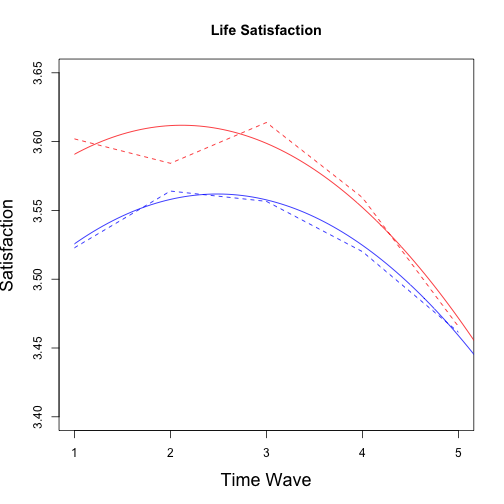
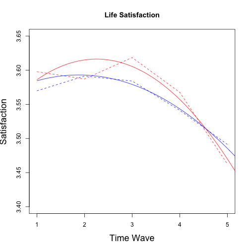
top CFA Growth - Life Satisfaction
## No growth vs. Linear
## chi: 60.37 ; df:2; p-value: 1.605e-12
## Linear vs. Quadratic
## chi: 55.4 ; df:2; p-value: 5.814e-11
## Quadratic vs. Cubic
## chi: 3.297 ; df:2; p-value: 0.2542
## Cubic vs. Quartic
## chi: 1.503 ; df:2; p-value: 0.5556
## Multiple imputation results:
##       MIcombine.default(betas, vars2)
##                    results       se   (lower   upper) missInfo
## (Intercept)      3.4606967 0.022016  3.41754  3.50386      3 %
## wave             0.0813027 0.015682  0.05055  0.11206      4 %
## group            0.0755141 0.048375 -0.01966  0.17068     12 %
## I(wave^2)       -0.0163273 0.002582 -0.02139 -0.01126      6 %
## wave:group      -0.0098441 0.035604 -0.08032  0.06063     19 %
## group:I(wave^2) -0.0005434 0.005847 -0.01213  0.01104     20 %
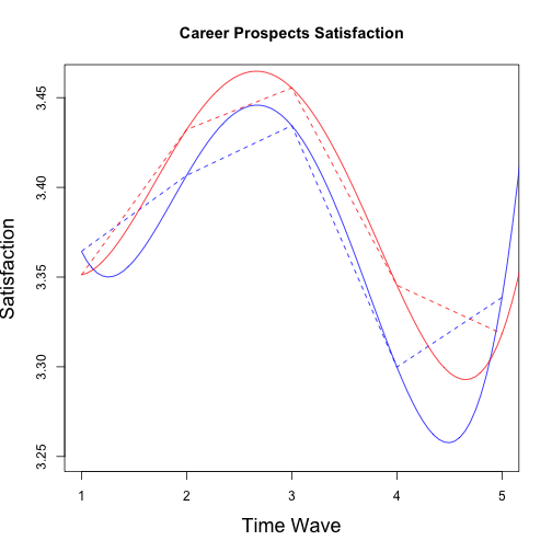
## No growth vs. Linear
## chi: 23.96 ; df:2; p-value: 5.693e-05
## Linear vs. Quadratic
## chi: 34.74 ; df:2; p-value: 1.075e-06
## Quadratic vs. Cubic
## chi: 31.17 ; df:2; p-value: 4.501e-07
## Cubic vs. Quartic
## chi: 28.08 ; df:2; p-value: 1.847e-05
## Multiple imputation results:
##       MIcombine.default(betas, vars2)
##                   results       se   (lower   upper) missInfo
## (Intercept)      3.938823 0.206495  3.52783  4.34981     24 %
## wave            -1.214167 0.380618 -1.97244 -0.45590     25 %
## group           -0.359440 0.441149 -1.24079  0.52191     27 %
## I(wave^2)        0.845665 0.229190  0.38860  1.30273     26 %
## I(wave^3)       -0.226104 0.055289 -0.33646 -0.11574     27 %
## I(wave^4)        0.020147 0.004612  0.01094  0.02936     27 %
## wave:group       0.636200 0.814495 -0.99334  2.26574     28 %
## group:I(wave^2) -0.373992 0.490465 -1.35635  0.60837     29 %
## group:I(wave^3)  0.092069 0.118456 -0.14549  0.32963     30 %
## group:I(wave^4) -0.008001 0.009909 -0.02790  0.01190     31 %
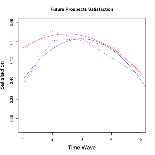
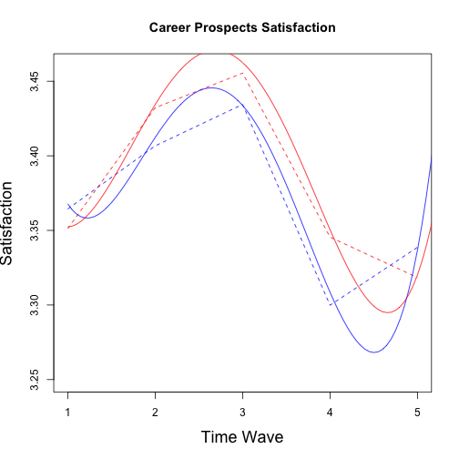
## No growth vs. Linear
## chi: 1.203 ; df:2; p-value: 0.5782
## Linear vs. Quadratic
## chi: 16.71 ; df:2; p-value: 0.001523
## Quadratic vs. Cubic
## chi: 1.974 ; df:2; p-value: 0.482
## Cubic vs. Quartic
## chi: 0.2884 ; df:2; p-value: 0.8882
## Multiple imputation results:
##       MIcombine.default(betas, vars2)
##                   results       se    (lower    upper) missInfo
## (Intercept)      3.346916 0.025336  3.296938  3.396895     15 %
## wave             0.064082 0.019087  0.026108  0.102056     24 %
## group            0.060824 0.054700 -0.047586  0.169233     21 %
## I(wave^2)       -0.010695 0.003194 -0.017082 -0.004308     28 %
## wave:group      -0.031779 0.042432 -0.117353  0.053796     34 %
## group:I(wave^2)  0.004211 0.007018 -0.009986  0.018408     35 %
## Matching equation used was:
##  group ~  W1WORK + W1LEISURE + W1GET.ALONG + W1WAGE + W1SOCIAL + W1INDEPENDENCE + W1CAREER.PROS + W1FUTURE.PROS + W1HOME.LIFE + W1LIVE.STAND + lbj003k + lbj003l + W1RESIDENCE + W1LIFE.SAT + W2WORK + W2LEISURE + W2GET.ALONG + W2WAGE + W2SOCIAL + W2INDEPENDENCE + W2CAREER.PROS + W2FUTURE.PROS + W2HOME.LIFE + W2LIVE.STAND + W2RESIDENCE + W2LIFE.SAT + W3WORK + W3LEISURE + W3GET.ALONG + W3WAGE + W3SOCIAL + W3INDEPENDENCE + W3CAREER.PROS + W3FUTURE.PROS + W3HOME.LIFE + W3LIVE.STAND + W3RESIDENCE + W3LIFE.SAT + sex + sisced + indig + laa005 + laa006 + escs + laa007 + laa025 + laa026 + laa027 + xcsl2003 + lad001 + belong + intmat + instmot + matheff + anxmat + scmat + complrn + cooplrn + teachsup + disclim + pv1math + pv1math1 + pv1math2 + pv1math3 + pv1math4 + pv1read + pv1scie + pv1prob + st30q01 + st30q02 + st30q03 + st30q04 + st30q05 + st30q06 + st30q07 + st30q08 + Sses + Smath + Sread + Sscie + Sprob
## R Version: R version 3.0.2 (2013-09-25)
## Library MatchIt loaded.
## Largest cohen's d differences for each imputation:
## ---------------------------------------------
## $m_mean_diff
## [1] -0.1894 -0.1343  0.1026  0.1010  0.1004
##
## $m_mean_diff
## [1]  0.1117 -0.1049
##
## $m_mean_diff
## [1] -0.1517 -0.1118  0.1038 -0.1006
##
## $m_mean_diff
## [1] -0.1012
##
## $m_mean_diff
## [1]  0.1295 -0.1080  0.1019
## Plot of mean differences pre and post matching
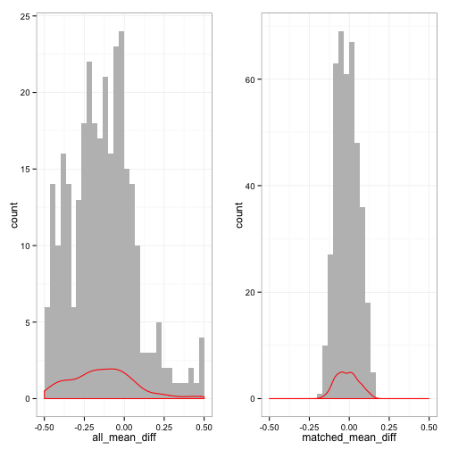
## cohen's d differences pre-matching:
##  Large Medium  Small
##  175.8  301.0 3008.2
## cohen's d differences post-matching:
## [1] 3485
## Total sample size: 1666
## Group sample size:
##  1183 482.4
## First year post univeristy
## ============================
## Univeristy enrolment
## ------------------
##               Direct   Gap
## Commenced      482.4 329.0
## Dropped out      0.0  11.6
## Not commenced    0.0 141.8
## Std. residuals: Cell
## ------------------
##               Direct    Gap
## Commenced      13.50 -13.50
## Dropped out    -3.42   3.42
## Not commenced -12.89  12.89
## p-value: 0.0004998
## Second year post univeristy
## ===========================
## Univeristy enrolment
## ------------------
##               Direct   Gap
## Commenced      425.6 329.8
## Completed        2.0   0.6
## Dropped out      1.0  13.8
## Not commenced   53.8 138.2
## Std. residuals: Cell
## ------------------
##         [,1]    [,2]
## [1,]  7.4851 -7.4851
## [2,]  0.9132 -0.9132
## [3,] -3.3578  3.3578
## [4,] -6.8100  6.8100
## p-value: 0.0004998
## Third year post univeristy
## ===========================
## Univeristy enrolment
## ------------------
##               Direct   Gap
## Commenced      403.2 320.4
## Completed       12.4  17.8
## Further Study    1.8   2.8
## Dropped out      2.8  22.8
## Not commenced   62.2 118.6
## Std. residuals: Cell
## ------------------
##                Direct     Gap
## Commenced      6.1599 -6.1599
## Completed     -0.9869  0.9869
## Further Study -0.5871  0.5871
## Dropped out   -4.0021  4.0021
## Not commenced -4.6590  4.6590
## p-value: 0.0004998
## Fourth year post univeristy
## ===========================
## Univeristy enrolment
## ------------------
##               Direct   Gap
## Commenced      266.8 202.6
## Completed      116.6 121.2
## Further Study   39.4  33.6
## Dropped out     14.2  36.0
## Not commenced   45.4  89.0
## Std. residuals: Cell
## ------------------
##                Direct     Gap
## Commenced      4.1364 -4.1364
## Completed     -0.3462  0.3462
## Further Study  0.7080 -0.7080
## Dropped out   -3.1625  3.1625
## Not commenced -4.0626  4.0626
## p-value: 0.0004998
## No growth vs. Linear
## chi: 75.38 ; df:2; p-value: 3.73e-14
## Linear vs. Quadratic
## chi: 30.52 ; df:2; p-value: 1.644e-05
## Quadratic vs. Cubic
## chi: 3.027 ; df:2; p-value: 0.2686
## Cubic vs. Quartic
## chi: 1.167 ; df:2; p-value: 0.6391
## Multiple imputation results:
##       MIcombine.default(betas, vars2)
##                   results       se     (lower    upper) missInfo
## (Intercept)      3.554056 0.029316  3.496e+00  3.612358     24 %
## wave             0.041538 0.020864 -9.719e-06  0.083085     25 %
## group           -0.035794 0.054303 -1.437e-01  0.072161     23 %
## I(wave^2)       -0.011051 0.003470 -1.799e-02 -0.004113     28 %
## wave:group       0.045626 0.042168 -4.016e-02  0.131407     38 %
## group:I(wave^2) -0.008311 0.007143 -2.299e-02  0.006372     43 %
## No growth vs. Linear
## chi: 18.99 ; df:2; p-value: 0.0004306
## Linear vs. Quadratic
## chi: 32.24 ; df:2; p-value: 9.153e-06
## Quadratic vs. Cubic
## chi: 20.32 ; df:2; p-value: 8.971e-05
## Cubic vs. Quartic
## chi: 16.44 ; df:2; p-value: 0.002261
## Multiple imputation results:
##       MIcombine.default(betas, vars2)
##                   results       se    (lower   upper) missInfo
## (Intercept)      3.847870 0.252364  3.343772  4.35197     27 %
## wave            -1.030895 0.470153 -1.973389 -0.08840     30 %
## group           -0.237482 0.482323 -1.207566  0.73260     32 %
## I(wave^2)        0.730410 0.284557  0.158585  1.30224     31 %
## I(wave^3)       -0.197258 0.068855 -0.335873 -0.05864     32 %
## I(wave^4)        0.017665 0.005755  0.006063  0.02927     33 %
## wave:group       0.394397 0.886452 -1.389156  2.17795     32 %
## group:I(wave^2) -0.222149 0.531387 -1.291346  0.84705     32 %
## group:I(wave^3)  0.054586 0.127959 -0.203026  0.31220     32 %
## group:I(wave^4) -0.004833 0.010682 -0.026360  0.01669     33 %
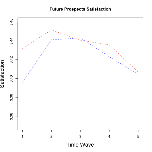
## No growth vs. Linear
## chi: 4.254 ; df:2; p-value: 0.1896
## Linear vs. Quadratic
## chi: 6.345 ; df:2; p-value: 0.08146
## Quadratic vs. Cubic
## chi: 1.418 ; df:2; p-value: 0.6013
## Cubic vs. Quartic
## chi: 0.7777 ; df:2; p-value: 0.7405
## Multiple imputation results:
##       MIcombine.default(betas, vars2)
##                results      se   (lower  upper) missInfo
## (Intercept)  3.4367483 0.01211  3.41272 3.46077     22 %
## group       -0.0003592 0.02125 -0.04219 0.04147     13 %